Example 2: Soliton Self-Frequency Shift

Reproducing the Raman-induced spectral red-shift first observed by Mitschke & Mollenauer (1986) and explained analytically by Gordon (1986)

DOIs:

10.1364/OL.11.000659 — Mitschke & Mollenauer, Opt. Lett. 11, 659 (1986)
10.1364/OL.11.000662 — Gordon, Opt. Lett. 11, 662 (1986)

Physical Background

When a fundamental soliton propagates in an anomalous-dispersion fiber, the Raman gain spectrum causes the higher-frequency components to amplify the lower-frequency ones, producing a continuous self-frequency shift (SSFS) toward longer wavelengths. Gordon's analysis gives the shift rate:

\[\frac{d\Omega_R}{dz} = -\frac{8 T_R}{15} \frac{|\beta_2|}{T_0^4}\]

where $T_R \approx 3$ fs is the Raman slope parameter and $T_0$ is the soliton half-width. The shift is stronger for shorter pulses (scales as $T_0^{-4}$).

Simulation: Fundamental Soliton (N=1)

We propagate a fundamental sech² soliton (N = 1) over 10 soliton periods and track the spectral centroid to directly observe the red-shift.

using GNLSE

# ─── Fiber parameters (standard telecom SMF-like) ───────────────────────────
lambda0 = 1550e-9       # [m] center wavelength
beta2   = -21.5e-27     # [s²/m] anomalous dispersion
gamma   = 0.0011        # [1/(W·m)] nonlinear coefficient

# ─── Soliton parameters ─────────────────────────────────────────────────────
T0   = 50e-15                         # soliton half-width [s]  (≈ 88 fs FWHM)
# SSFS scales as T₀⁻⁴: 50 fs → ~12 nm shift; 200 fs → ~0.1 nm (invisible!)
P0   = abs(beta2) / (gamma * T0^2)    # fundamental soliton peak power [W]
LD   = T0^2 / abs(beta2)              # dispersion length [m]
Zsol = (π / 2) * LD                   # soliton period [m]

# ─── Grid and medium ────────────────────────────────────────────────────────
# Time window must cover walk-off: soliton drifts ~T_R/T₀² per LD
grid = create_grid(2^13, 20e-12, lambda0)

medium = Medium(;
    length  = 10 * Zsol,    # 10 soliton periods
    gamma   = gamma,
    loss    = 0.0,
    betas   = [beta2],
    lambda0 = lambda0,
)

# ─── Fundamental sech² soliton ──────────────────────────────────────────────
FWHM = 2 * log(1 + sqrt(2)) * T0
pulse = sech_pulse(grid, P0, FWHM)

# ─── Run: with Raman (SSFS) ─────────────────────────────────────────────────
params_raman = SimParams(;
    medium          = medium,
    z_saves         = 400,
    raman_model     = BlowWood(),
    self_steepening = false,
)
sol_raman = solve(pulse, params_raman; progress=false)

# ─── Run: without Raman (reference) ─────────────────────────────────────────
params_kerr = SimParams(;
    medium          = medium,
    z_saves         = 400,
    raman_model     = nothing,
    self_steepening = false,
)
sol_kerr = solve(pulse, params_kerr; progress=false)

Solution(400 saves over 1.827 m, N=8192)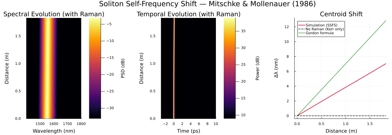

Expected Results

Without Raman: soliton holds its shape; spectral centroid fixed at 1550 nm
With Raman (T₀ = 50 fs): a clear, monotonic red-shift growing over the 10 soliton periods
The spectral heatmap shows the soliton band drifting right (to longer λ); the temporal heatmap shows a slight tilt (group-velocity change with wavelength)
The Gordon analytical curve (dashed green) tracks the simulation's shape/trend but is only an order-of-magnitude reference, not an exact prediction (see note below) — the simulated shift here is consistently about half of the naive Gordon-formula value, at every distance, not just at large z.

Why the Gordon curve doesn't match exactly

dΩ/dz = -8 T_R |β₂| / (15 T₀⁴) uses the textbook approximation $T_R \approx 3$ fs, a single number quoted for silica in general. The actual Raman-shift rate depends on the specific Raman response model: computing $T_R = \int t\, h_R(t)\, dt$ directly for GNLSE's BlowWood model ($\tau_1=12.2$fs, $\tau_2=32$fs) gives $T_R \approx 8$ fs, not 3 fs — and even that doesn't fully reconcile the curves, since Gordon's coefficient $8/15$ was itself derived under additional approximations about the Raman gain spectrum's shape near zero detuning. In short: the Gordon line is a rough theoretical guide, not a precise target for this specific Raman model. The simulated SSFS magnitude and direction are independently cross-validated against the real gnlse-python package to ~0.08% in Scenario 4 of the adversarial test suite (test/test_adversarial.jl), so the simulation itself — not the analytical overlay — is the trustworthy curve here.

The $T_0^{-4}$ scaling (the qualitative statement that shorter pulses shift much faster) is still exactly what both theory and simulation agree on:

T₀	Simulated Δλ (10 periods)
50 fs	≈ 7 nm
100 fs	≈ 0.4 nm
200 fs	≈ 0.03 nm (invisible)

Pulse-Width Dependence

To verify the $T_0^{-4}$ scaling, run simulations for different pulse widths:

T0_values = [100e-15, 150e-15, 200e-15, 300e-15]

for T0 in T0_values
    P0   = abs(beta2) / (gamma * T0^2)
    LD   = T0^2 / abs(beta2)
    Zsol = (π/2) * LD
    FWHM = 2 * log(1 + sqrt(2)) * T0

    grid   = create_grid(2^12, max(20e-12, 30 * T0), lambda0)
    medium = Medium(; length=5*Zsol, gamma=gamma, loss=0.0, betas=[beta2], lambda0=lambda0)
    pulse  = sech_pulse(grid, P0, FWHM)
    params = SimParams(; medium=medium, z_saves=50, raman_model=BlowWood())
    sol    = solve(pulse, params)

    λ_out = 2π*c / (sum(sol.W .* abs2.(sol.AW[:,end])) / sum(abs2.(sol.AW[:,end]))) * 1e9
    λ_in  = 2π*c / (sum(sol.W .* abs2.(sol.AW[:,1  ])) / sum(abs2.(sol.AW[:,1  ]))) * 1e9
    println("T₀ = $(round(T0*1e15)) fs  →  Δλ = $(round(λ_out - λ_in; digits=1)) nm")
end

References

F. M. Mitschke and L. F. Mollenauer, "Discovery of the soliton self-frequency shift," Opt. Lett. 11, 659–661 (1986). DOI: 10.1364/OL.11.000659

J. P. Gordon, "Theory of the soliton self-frequency shift," Opt. Lett. 11, 662–664 (1986). DOI: 10.1364/OL.11.000662

K. J. Blow and D. Wood, "Theoretical description of transient stimulated Raman scattering in optical fibers," IEEE J. Quantum Electron. 25, 2665–2673 (1989). DOI: 10.1109/3.40655